In drone mapping and search and rescue (SAR), ground sample distance (GSD) is the distance between adjacent pixel centers measured on the ground. In a digital photograph with a 1-meter GSD, such as U.S. National Agriculture Imagery Program (NAIP) aerial imagery, adjacent pixel locations sit 1 meter apart on the surface. At a vertical nadir view looking straight down, GSD equals height above ground level times physical pixel pitch, divided by lens focal length: GSD = (h x p) / f.
Because GSD describes the ground width of a single pixel, it measures only one limitation on spatial resolution, namely the limitation due to sampling. NC State Extension separates image resolution, expressed as horizontal pixels times vertical pixels across the frame, from ground sampling distance, which translates each pixel into physical dimensions on the ground. Cal Poly Humboldt’s aerial photography lesson notes that a digital sensor is defined by three distinct properties: its physical size, the dimension of its pixels, and the number of pixels in the sensor.
How Is Ground Sample Distance Calculated at Nadir?
At a straight-down nadir view, horizontal offset from vertical is zero, slant range equals flying height above ground level (h), and the slant angle from nadir (theta) is 0 degrees, whose cosine is 1. Wikipedia simplifies the imaging geometry to GSD = (h x p) / f, where p = P / N is physical pixel size, P is the physical width or height of the sensor, N is the total number of pixels in that same sensor dimension, and f is the camera lens focal length. U.S. Bureau of Land Management (BLM) photogrammetric guidance writes the same relation as GSD = SPS * H / f, computing Sensor Pixel Size (SPS) by dividing the physical width of the sensor by the width of the sensor in pixels.
Three input checks prevent unit and datum errors before a flight:
- Use height above ground level (AGL) rather than altitude above sea level. Cal Poly Humboldt notes that estimating AGL requires subtracting the average elevation of the terrain from altitude above sea level, and NC State Extension notes that flying lower decreases GSD if all other sensor parameters stay the same.
- Use the lens’s real focal length. Digital cameras may list both a 35 mm equivalent focal length and a real focal length, and Cal Poly Humboldt specifies using the real focal length when determining GSD.
- Convert focal length and pixel pitch to one shared linear unit before dividing. Pennsylvania State University’s flight-planning lesson notes that when focal length (f) and pixel size (ab) are converted to the same linear unit, the resulting flying altitude comes out in the same linear unit as the GSD.
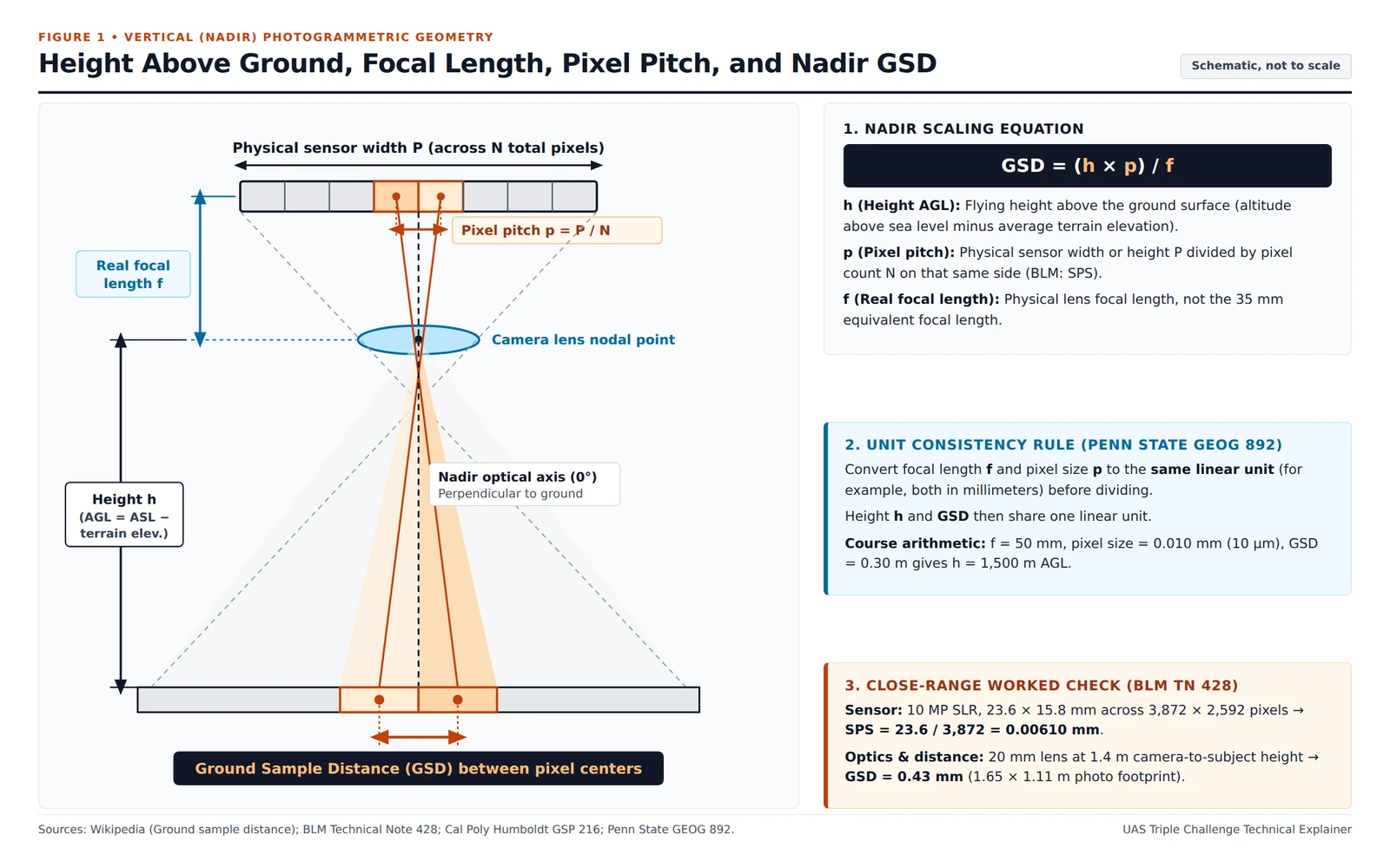
Nadir camera geometry maps adjacent detector centers separated by pixel pitch p = P / N through real focal length f across height h above ground level onto ground sample centers.
Published government and university examples show how consistent units work across a close-range subject, a flight-planning course example, and a public imagery reference:
| Published Source | Sensor and Pixel Pitch | Focal Length and Distance | Resulting GSD and Scope |
|---|---|---|---|
| U.S. Bureau of Land Management photogrammetric note | 10 megapixel SLR, 23.6 x 15.8 mm sensor, 3,872 x 2,592 pixels; SPS = 23.6 / 3,872 = 0.00610 mm | 20-mm lens at 1.4 m camera height above the subject | 0.43 mm GSD across a 1.65 x 1.11 m photo footprint (close-range subject distance, not an aircraft search altitude) |
| Pennsylvania State University flight-planning lesson | Pixel size ab = 0.010 mm (10 um) | f = 50 mm at 1,500 meters flying height above ground level | 0.30 meter GSD (university flight-route course example, not a small-UAS search altitude) |
| Cal Poly Humboldt aerial photography lesson | NAIP imagery | Imagery resolution stated by the lesson | 1-meter ground sample distance |
How Do Nadir and Oblique Angles Change Ground Sample Distance?
Cal Poly Humboldt classifies aerial photographs taken looking straight down as vertical photographs and any aerial photographs taken at an angle as oblique photographs: low-oblique frames show only the surface without the horizon, whereas high-oblique frames show the surface, the horizon, and a portion of sky. BLM photogrammetric guidance states that imagery taken as close to nadir (perpendicular to the subject) as possible is most desirable, with the plane of the sensor and lens kept parallel to the subject to maintain a consistent height or distance. When terrain or project size makes nadir photography impractical, oblique photography is used and camera distance can be interchanged for camera height, though BLM notes that a sharp low-angle oblique camera angle should be avoided unless necessary to provide stereo overlap.
When the sensor points off nadir, Wikipedia gives the oblique ground sample distance as slant range times physical pixel size p, divided by focal length f times cos(theta). In that geometry, slant range equals sqrt(d^2 + h^2), where d is horizontal offset from nadir, h is height above ground level, and theta = arctan(d / h) is the slant angle measured from 0 degrees at nadir. Dividing by cos(theta) accounts for the oblique viewing angle, which increases the effective ground footprint of each pixel; written directly in terms of horizontal offset d and height h, Wikipedia expresses this planar relation as GSD = ((d^2 + h^2) / h) x (p / f).
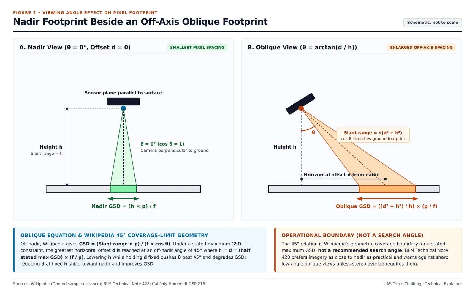
Off-nadir viewing increases both slant range to the ground and oblique footprint projection via cos(theta), enlarging ground sample spacing compared with a vertical nadir view at the same height h.
Under a specified maximum GSD constraint, Wikipedia shows that the greatest horizontal distance d is achieved at a 45 degree off-nadir angle where height h equals horizontal distance d, giving d = h equal to half that specified maximum GSD times (f / p). Reducing horizontal distance d without lowering height h decreases the off-nadir angle toward nadir and improves GSD, whereas decreasing height h while keeping d constant increases the off-nadir angle beyond 45 degrees and degrades GSD. That 45 degree configuration represents Wikipedia’s widest horizontal coverage geometry for a specified maximum GSD constraint rather than a recommended search camera angle.
Why Does GSD Differ from Spatial Resolution and Map Accuracy?
Sample spacing on the detector grid and resolved detail in the recorded frame are distinct physical quantities. A NASA spatial-resolution review defines ground sampling distance as the separation between centers of two adjacent samples on the ground, while defining Sensor Spatial Resolution (SSR) as the full-width at half-maximum (FWHM) of the sensor line spread function (LSF) projected on the ground. That same NASA review defines Ground Resolved Distance (GRD) as the effective sensor resolution equal to the half wavelength on the ground where the modulation transfer function (MTF) of the line spread function drops to 1/2, noting that GRD is affected by system blur.
Camera motion and exposure duration also constrain usable detail alongside pixel geometry. For handheld close-range photography, BLM photogrammetric guidance states that a shutter speed of at least 1/200th of a second is required, and camera motion from wind or an unstable platform such as a ladder may make high shutter speeds (more than 1/1,000th of a second) necessary. Phase One’s photogrammetric support documentation similarly notes that GSD depends on focal length, sensor resolution, sensor size, and distance to the ground, and that its calculators also take motion blur due to ground speed into account.
Smaller pixels also do not guarantee survey-grade coordinates. U.S. Geological Survey (USGS) UAS imagery calibration guidance states that ground control point (GCP) accuracy needs to be at least three times the required accuracy of UAS imagery, so the accuracy of the UAS data has no direct relation with the GSD of the pixels. In the USGS report’s example, a dataset with a 1-centimeter (cm) GSD may well have an accuracy of less than 6 cm at 1 sigma if the GCPs have an accuracy of 2 cm or less at 1 sigma. USGS cautions users not to assign higher accuracy to UAS imagery just because the GSD is lower, while noting that a lower GSD allows the user to identify documented and other targets on the ground, which helps achieve higher accuracy for the data.
How Many Pixels and Line Pairs Discriminate a Target?
NC State Extension notes that at least two pixels are needed to describe a target from above, although a greater number of pixels helps increase resolution. Flying lower to improve GSD means that more pictures are needed to cover the area, whereas a higher flight needs fewer images to cover the same area. How extra flight lines interact with battery weight and airborne endurance is covered in our guide on the drone payload capacity and flight-time degradation curve, how parallel track spacing and sweep width govern area coverage is detailed in search grid patterns and probability of detection, and how containment and detection probabilities combine under tree canopy appears in our UAS search optimization explainer. Readers tracking how first-responder forest search trials framed onboard image detection can consult the UAS Triple Challenge archive and related technical guides in Topics.
For visual target discrimination, John Johnson created the Johnson criteria in 1958 to calculate the probability of detection of an object imaged by an optical system, and a Sandia National Laboratories historical review notes that the criteria are not exclusively military and can be used where a person is looking for a specific target in a static or moving image. Sandia defines the Johnson criteria as the number of cycles across a target for an ensemble of observers to have a 50% chance of completing the discrimination task:
| Discrimination Task | Sandia Cycle Count (50% Ensemble Observer Chance) | Wikipedia Line-Pair Threshold and Task Description |
|---|---|---|
| Detection | 1.0 +/- 0.25 cycles: object is of military significance | 1.0 +/- 0.25 line pairs: an object is present |
| Orientation | 1.4 +/- 0.35 cycles: object aspect | 1.4 +/- 0.35 line pairs: symmetrical, asymmetric, horizontal, or vertical |
| Recognition | 4.0 +/- 0.8 cycles: class of object (jeep or tank) | 4 +/- 0.8 line pairs: the type of object can be discerned, a person versus a car |
| Identification | 6.4 +/- 1.5 cycles: member of class | 6.4 +/- 1.5 line pairs: a specific object can be discerned, a woman versus a man, or the specific car |
Wikipedia notes that Johnson’s line pairs refer to lines displayed on an interlaced CRT monitor. Each line pair corresponds to 2 pixels of a film image, or an image displayed on an LCD monitor.
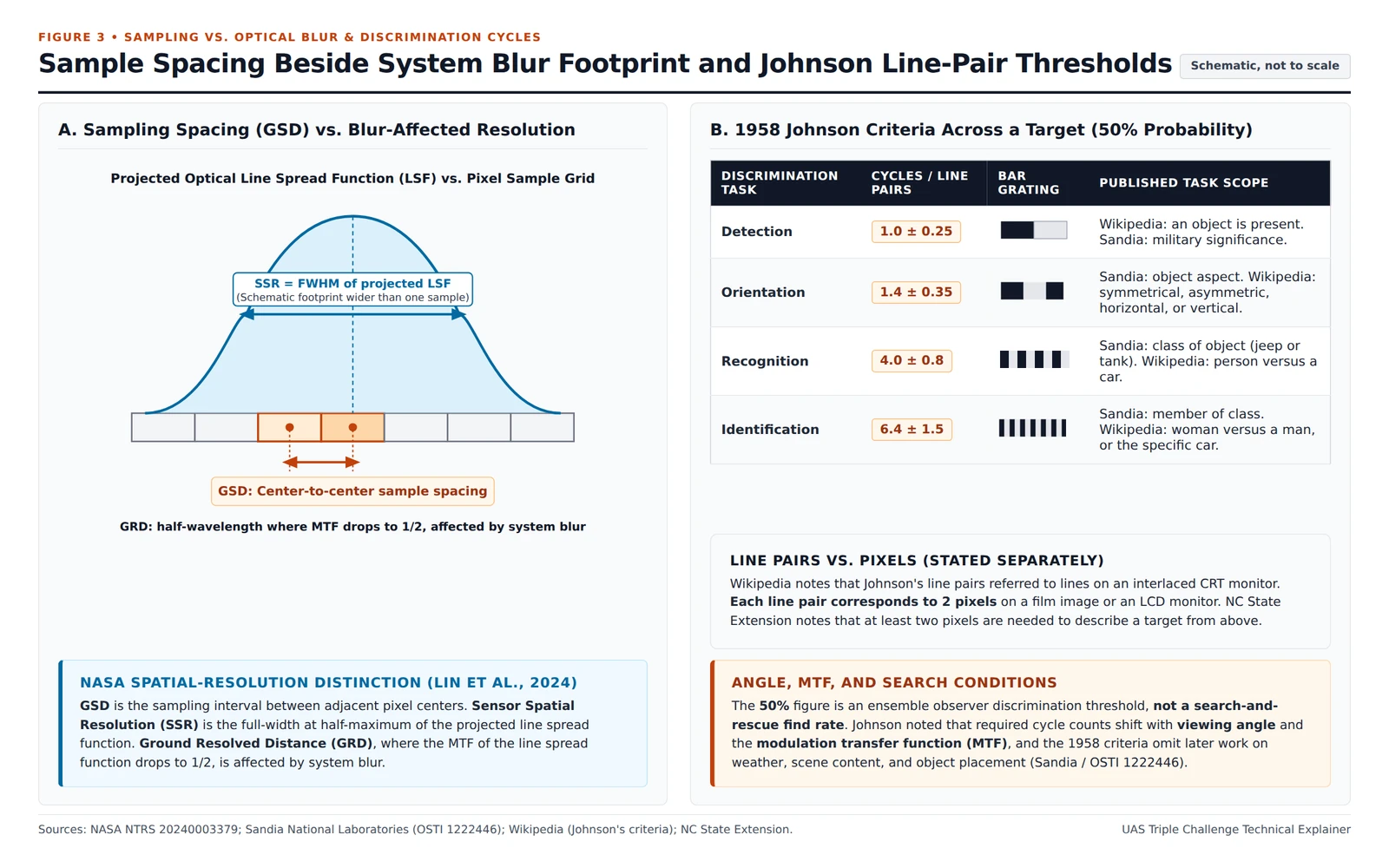
System blur affects the projected line spread function and Ground Resolved Distance, drawn here as a wider footprint than one sample spacing, while Johnson’s 1958 observer discrimination thresholds change with viewing angles and the modulation transfer function.
Johnson recognized that these cycle counts change based on viewing angles and the contrast transfer function, also called the modulation transfer function. Sandia’s review notes that the initial 1958 criteria do not reflect later target-acquisition research into weather, scene content, and object placement. The 50% figure in those tables is an ensemble observer discrimination threshold rather than a field search-and-rescue find rate.
Pre-Flight GSD and Resolution Review Sheet for Mapping and Search Legs
Before launching a mapping pass or visual search leg, verify each optical and geometric input in consistent linear units:
| Pre-Flight Check Item | Input or Relation to Verify | Operational Check Purpose |
|---|---|---|
| Height above ground level (h / AGL) | Subtract average terrain elevation from altitude above sea level rather than entering sea-level altitude | Keeps ground pixel spacing tied to surface clearance |
| Real lens focal length (f) | Enter the camera’s real focal length rather than any 35 mm equivalent focal length | Prevents false GSD estimates from 35 mm equivalent numbers |
| Physical pixel pitch (p or SPS) | Divide physical sensor width or height P by pixel count N along that same dimension in the same linear unit as f | Grounds calculations in physical pixel size rather than pixel count alone |
| Nadir sample spacing and image count | Compute GSD = (h x p) / f at 0 degrees and account for more pictures needed when flying lower | Balances target pixel spacing against total frames across the area |
| Off-nadir slant angle (theta) or offset (d) | Apply ((d^2 + h^2) / h) x (p / f) for oblique camera tilt; keep views near nadir unless terrain or stereo overlap requires oblique imagery | Accounts for off-axis footprint stretching from slant range and cos(theta) |
| Shutter check against one ground sample | Check shutter speed against wind, unstable mounts, and ground speed (BLM: at least 1/200th s handheld, more than 1/1,000th s in wind or on an unstable platform) | Keeps camera motion blur from degrading Ground Resolved Distance across adjacent samples |